Steady-State Concentration: Principles, Calculations, and Clinical Application

Steady state is a cornerstone concept in clinical pharmacokinetics. It connects dose, dosing interval, and patient-specific clearance to the drug concentrations that drive therapeutic and adverse effects. Yet, “steady state” is often misunderstood or oversimplified. This chapter explains what steady state is (and is not), how it arises under different dosing schemes, how to calculate and predict steady-state concentrations, and how to apply these ideas to individualized dosing and therapeutic drug monitoring (TDM). We highlight linear versus nonlinear behavior, infusion versus intermittent dosing, accumulation, fluctuation, loading doses, and special scenarios such as long-acting formulations, critical illness, and altered protein binding.

Key takeaways

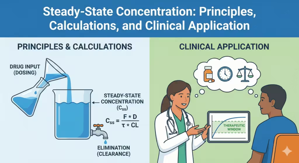
• Steady state exists when, under time-invariant conditions, the concentration–time profile repeats identically each dosing interval; input equals elimination over each cycle [1–3].
• For linear kinetics, average steady-state concentration (Css,avg) depends only on dose rate and clearance: Css,avg = (F × Dose/τ)/CL or, for infusion, Css = R0/CL [1,2].
• Time to steady state depends on elimination half-life (t1/2), not dose: about 4–5 half-lives to approach >90–97% of steady state [1–3].
• Accumulation and fluctuation are governed by the relationship between dosing interval (τ) and half-life; longer τ increases peak–trough variation [1,3,4].
• Nonlinear or time-varying kinetics (e.g., saturation, autoinduction) shift steady state and invalidate simple linear predictions [1,2].
• In clinical care, sample at or near steady state when using concentration targets, and consider unbound drug when protein binding is altered [3,5].

Defining Steady State

What steady state means

Steady state is achieved during multiple dosing or continuous infusion when the amount of drug entering the body per unit time equals the amount eliminated per unit time, given constant pharmacokinetic parameters (clearance, volume, bioavailability). At that point, concentrations over each dosing interval repeat in a stable pattern: same peak, trough, and area under the curve (AUC) each cycle [1–3].

Important nuances:

• Steady state is a dynamic equilibrium: continuous input and elimination, not stasis.
• It refers to the entire periodic concentration–time profile, not a single number (unless infusion, where concentration becomes constant after sufficient time).
• It requires time-invariant PK; if clearance or bioavailability changes (enzyme induction, organ failure), the steady state shifts [1,2].

Distinguishing average, peak, and trough at steady state

• Css,avg (average over a dosing interval) is the primary exposure metric linking dose rate and clearance.
• Cmax,ss and Cmin,ss are the steady-state peak and trough; they depend on both clearance and the dosing interval relative to half-life (fluctuation) and on absorption rate for extravascular dosing [1–3].

Mathematical Foundations

Linear kinetics and superposition

For most dose ranges, many drugs follow linear (first-order) kinetics: pharmacokinetic parameters are constant, and exposure (AUC) is proportional to dose. Multiple dosing and infusion can be handled using superposition: the total concentration is the sum of individual single-dose contributions shifted by integer multiples of the dosing interval [1–3].

Key linear relations:

• Css,avg = (F × Dose/τ)/CL
• AUC over one steady-state interval (AUCτ,ss) = F × Dose/CL (same as single-dose AUC for IV the relationship AUC = Dose/CL)
• Fraction of steady state reached after time t (infusion or repeated dosing) = 1 − e^(−k × t), where k = ln(2)/t1/2 [1–3].

Time to steady state and accumulation

• Time to steady state depends only on elimination half-life. Typical rules of thumb:
• 50% steady state at 1 half-life; 75% at 2; ~87.5% at 3; ~94% at 4; ~97% at 5 so typically it takes 4 to 5 plasma half-life.
• Accumulation ratio (Racc) for intermittent dosing in a one-compartment model:
• Racc = 1 / (1 − e^(−k × τ))
• Intuition: shorter τ relative to half-life produces greater accumulation [1,3,4].

Fluctuation at steady state

Fluctuation is the ratio of peak to trough within a dosing interval. For one-compartment IV bolus dosing:

• Cmax,ss/Cmin,ss = e^(k × τ)
  Thus, for a given half-life, shortening the dosing interval reduces fluctuation (more even concentrations), while lengthening it increases fluctuation [1–3].

Steady State Under Different Dosing Schemes

Continuous IV infusion

• Concentration during infusion: C(t) = Css × [1 − e^(−k × t)], where Css = R0/CL and R0 is the infusion rate.
• Time to reach a fraction of Css follows the half-life rules above (no peaks/troughs once at steady state).
• Stopping infusion leads to mono-exponential decline: C(t) = Css × e^(−k × t) [1–3].

Clinical strategies:

• Use a loading dose to reach Css rapidly, then continue infusion to maintain it (see Loading Doses).
• For narrow therapeutic index drugs with short half-lives (e.g., some anesthetics), infusion enables tight control [1,2].

Intermittent IV bolus dosing

• After many doses, the profile stabilizes: the peak right after dosing, and the trough just before the next dose, repeat each interval.

For a one-compartment model with immediate distribution:

• Cmax,ss ≈ (Dose/V) × [1/(1 − e^(−k × τ))]
• Cmin,ss = Cmax,ss × e^(−k × τ)
• Css,avg still equals (Dose/τ)/CL because AUCτ,ss = Dose/CL [1–3].
• In multicompartment kinetics, early post-dose concentrations reflect distribution phases; “peak” sampling too early may overestimate pharmacologic exposure [1,2].

Repeated oral dosing

• Css,avg = (F × Dose/τ)/CL remains valid under linear kinetics.
• The absorption rate constant (ka) shapes peak/trough amplitudes:
• Rapid absorption (ka >> k) yields sharper peaks/higher fluctuation.
• Slower absorption (ka closer to k) smooths the profile (lower peaks, higher troughs), often reducing fluctuation at the same average exposure [1–3,4].
• Flip-flop kinetics (ka < k) make the terminal slope reflect absorption rather than elimination; apparent half-life is absorption-limited, affecting time to steady state and accumulation. Long-acting oral/depot formulations often behave this way [2,3].

Loading Doses and Maintenance

Why and when to load

Without a loading dose, it takes ~4–5 half-lives to approach steady-state levels—sometimes too slow for urgent indications (e.g., antiepileptics, immunosuppressants, serious infections). A loading dose raises concentrations to the target range quickly; ongoing maintenance dosing then keeps them there [1,2].

Calculating loading doses

• IV bolus (one-compartment approximation): LD = target concentration × V
• Oral or other extravascular: LD = (target concentration × V)/F
• Continuous infusion: give LD ≈ Css,target × V, then start infusion at R0 = CL × Css,target
• For multicompartment drugs, a single bolus may cause transient overshoot in the central compartment. Split or “primed infusion” strategies can temper early peaks [1–3].

Practical cautions:

• V should reflect the apparent volume relevant to the sampling compartment and timing (Vss is a common choice for steady-state targets).
• If binding is concentration-dependent (e.g., valproate), targeting unbound concentrations is safer (see Protein Binding) [5].

Nonlinear and Time-Dependent Kinetics

Saturation (capacity-limited) kinetics

At higher concentrations, enzymes, transporters, or binding sites may saturate:

• Michaelis–Menten elimination (e.g., phenytoin): clearance decreases as concentrations rise; small dose increases can cause disproportionate concentration jumps, and a unique “steady state” may not exist if maintenance dose exceeds maximal elimination capacity [1,2].
• Saturable protein binding (e.g., valproate): unbound fraction increases with concentration, altering both distribution and elimination [2,5].

Clinical implications:

• Avoid large dose escalations near the nonlinear range; titrate slowly and rely on TDM.
• Average steady-state relations (Css,avg = Dose rate/CL) do not hold; use patient-specific models or validated nomograms [1,2].

Time-dependent clearance

• Autoinduction (e.g., carbamazepine) increases clearance over days to weeks; steady-state concentrations decline unless dose is adjusted.
• Mechanism-based inhibition (quasi-irreversible enzyme inhibition) decreases clearance until enzyme resynthesis occurs, raising concentrations [2].
• Inflammation, organ function changes, or interacting drugs can shift steady state during therapy.

Management:

• Anticipate time trends; schedule follow-up levels after induction/inhibition reaches new equilibrium.
• Adjust doses iteratively or use model-informed approaches [1,2].

Unbound Concentrations and Protein Binding

Unbound at steady state

Pharmacologic effect and clearance are driven by unbound drug. For linear binding:

• Css,u,avg = fu × Css,avg (fu is unbound fraction).
• Changes in plasma protein binding alter total concentrations, but often not unbound exposure and effect, especially for high-extraction or flow-limited clearance drugs [5].
• In conditions altering albumin or alpha-1-acid glycoprotein (critical illness, hepatic disease, inflammation), consider measuring free levels for narrow therapeutic index drugs (e.g., phenytoin) [2,5].

Designing Regimens: Fluctuation, Interval, and Targets

Choosing the dosing interval (τ)

Trade-offs:

• Short τ: lower fluctuation, potentially better tolerability, but more frequent dosing burden.
• Long τ: higher fluctuation; for drugs with concentration-related toxicity or efficacy thresholds, this can be problematic.

Rules of thumb:

• Aim for τ ≈ t1/2 to balance fluctuation and convenience if peaks and troughs both matter.
• For time-dependent killers (antibiotics where fT>MIC predicts efficacy), use shorter τ or extended/continuous infusion to raise time above MIC at similar average exposure [6–8].
• For concentration-dependent drugs (Cmax/MIC or AUC/MIC drivers), allow more fluctuation if peaks are beneficial and tolerated [6–8].

Target exposure strategies

• Target concentration intervention: choose LD and maintenance dose to attain a specific Css,target or AUC target, then verify with TDM [9].
• AUC-guided dosing: increasingly favored for vancomycin (AUC24/MIC 400–600 mg·h/L) using Bayesian methods at or near steady state [10].
• Trough-based dosing: acceptable for some drugs (e.g., tacrolimus) where trough correlates with exposure and effect, but AUC-based methods may be superior when feasible [2].

Therapeutic Drug Monitoring at Steady State

When and what to sample

• Sample after steady state is reached, unless assessing loading or emergent toxicity.

Choose sampling times to inform the target metric:

• Troughs for trough-based targets (immunosuppressants).
• Two timed samples within a dosing interval for Bayesian AUC estimation (e.g., vancomycin).
• Peaks/troughs for aminoglycosides in extended-interval dosing (Cmax/MIC; near-zero troughs to limit toxicity) [10,11].
• Confirm assay methods and timing relative to dose (document exact times): small timing errors can mislead interpretation near peaks [2,11].

Bayesian forecasting and model-informed precision dosing

Combining prior population PK with one or two patient concentrations yields individualized parameter estimates and dose recommendations aimed at a target exposure (Css,avg, AUC, or Cmax/MIC). This improves target attainment and may reduce toxicity, especially in variable populations (children, critically ill) [3,12].

Special Situations Influencing Steady State

Long-acting and depot formulations

• Absorption-limited (flip-flop) kinetics: the apparent half-life reflects slow absorption, so time to steady state and accumulation are driven by the absorption process.
• Loading can be achieved with an initial immediate-release dose or “front-loaded” depot schedules.
• Missed doses may have delayed consequences; dose replacement strategies depend on time since last injection and absorption kinetics [2,3].

Critical illness and augmented renal clearance (ARC)

• In some ICU patients, glomerular filtration is increased (ARC), raising clearance and reducing Css,avg for renally eliminated drugs at standard doses.
• Capillary leak, fluid shifts, and altered protein binding can change V and the time to reach steady state; TDM and model-informed dosing are often needed (e.g., beta-lactams, vancomycin) [13,14].

Renal and hepatic impairment

• Reduced renal function lowers clearance of renally eliminated drugs; at a fixed dose rate, Css,avg increases and time to steady state lengthens. Adjust dose rate (Dose/τ) proportional to the change in clearance or extend τ to control troughs [2].
• Hepatic impairment can alter blood flow, intrinsic clearance, and protein binding; net effects depend on extraction ratio and binding. Empirical PK studies and labeling guide dose adjustments [2].

Adherence and missed doses

• At steady state, skipping a single dose allows concentration to decay for an additional τ; the impact depends on k and τ:
• Roughly, trough falls by a factor e^(−k × τ) more than expected at the next scheduled time.
• If maintaining trough above a threshold is critical (anticonvulsants, immunosuppressants), counsel on adherence and consider formulations or intervals that reduce fluctuation.
• For accidental extra doses, the temporary peak rise depends on residual concentration; assess toxicity risk based on peak-related adverse effects and half-life [2,15].

Worked Logic Without Heavy Math

From target to dose

• Goal: Css,avg,target
• Choose: maintenance dose rate = CL × Css,avg,target
• For oral: Dose per interval = (CL × Css,avg,target × τ)/F
• For infusion: R0 = CL × Css,avg,target
• If quick effect needed: LD ≈ Css,target × V (IV) or divide by F for oral
• Verify with TDM at steady state; adjust using observed concentrations and Bayesian tools if available [1–3,10,12].

Balancing fluctuation and convenience

• If peaks cause toxicity: shorten τ or use extended/continuous infusion.
• If high peaks improve efficacy: allow longer τ provided troughs remain adequate.
• Always check that Css,avg meets the exposure target; do not rely on half-life alone to judge adequacy [1–3].

Common Pitfalls

Misinterpreting half-life

Half-life dictates time to steady state and fluctuation for a given τ, but not average exposure. Only clearance sets Css,avg at a given dose rate. Changing interval without changing dose rate can keep Css,avg constant while altering peaks and troughs [1–3].

Assuming linearity near saturation

For drugs like phenytoin, small dose increases can cause large concentration jumps once near Km; steady-state predictions from linear formulas fail. Use cautious titration and TDM [1,2].

Ignoring protein binding changes

Total concentrations may fall when albumin is low, yet unbound (active) levels remain the same or increase. Dose to effect/unbound targets when binding is altered or variable; interpret total levels in context [5].

Sampling too early post-dose

In multicompartment kinetics, “peaks” sampled during distribution phases can misrepresent pharmacodynamic exposure. Follow drug-specific TDM timing recommendations [2,11].

Practical Checklist

Before prescribing

• Define exposure target (Css,avg, AUC/MIC, trough).
• Estimate CL and V from population data and patient factors (size, eGFR, hepatic function).
• Choose τ based on half-life, target fluctuation, and feasibility.
• Calculate LD and maintenance dose rate; plan TDM timing.

During therapy

• Sample at or near steady state and at appropriate times (trough, timed pairs).
• Use Bayesian tools when possible to refine CL and V.
• Reassess with changes in organ function, interacting drugs, or clinical status.
• Educate on adherence; document dose times and sampling times precisely.

Short Clinical Examples

Vancomycin

• Target AUC24/MIC 400–600 mg·h/L in serious MRSA infections.
• Start with LD (25–30 mg/kg actual body weight) to approach target sooner; estimate maintenance dose rate from renal function and population CL.
• Use Bayesian AUC monitoring within first 24–48 h (not necessarily full steady state) and re-estimate as renal function stabilizes [10,13].

Aminoglycosides (extended-interval)

• Concentration-dependent killing favors higher Cmax/MIC; long τ allows low troughs to minimize toxicity.
• Use nomograms or Bayesian tools to set τ and dose; verify levels to adjust for ARC or renal impairment [11,13,14].

Phenytoin

• Nonlinear elimination; steady state may be reached slowly and unpredictably as concentrations approach Km.
• Use small dose adjustments and measure total and free concentrations when albumin is low [1,2,5].

Conclusion

Steady state is the kinetic equilibrium that links dose rate to exposure and, ultimately, clinical response. Under linear, time-invariant conditions, its logic is simple: average exposure equals dose rate divided by clearance; half-life dictates how quickly steady state is reached and how much concentrations fluctuate between doses. Real patients add complexity—nonlinear or time-dependent processes, variable protein binding, organ dysfunction, critical illness, and adherence—all of which can shift steady state or complicate its attainment. A disciplined approach—clear exposure targets, rational interval selection, thoughtful use of loading doses, and verification with appropriately timed TDM, ideally via Bayesian methods—translates steady-state theory into safer, more effective therapy.

References

1. Rowland M, Tozer TN, Derendorf H, Hochhaus G. Clinical Pharmacokinetics and Pharmacodynamics: Concepts and Applications. 5th ed. Philadelphia (PA): Wolters Kluwer; 2019.
2. Shargel L, Wu-Pong S, Yu ABC. Applied Biopharmaceutics & Pharmacokinetics. 7th ed. New York (NY): McGraw-Hill; 2015.
3. Gabrielsson J, Weiner D. Pharmacokinetic and Pharmacodynamic Data Analysis: Concepts and Applications. 5th ed. Stockholm (SE): Swedish Pharmaceutical Press; 2016.
4. Benet LZ, Kroetz DL, Sheiner LB. Pharmacokinetics: The Dynamics of Drug Absorption, Distribution, and Elimination. In: Hardman JG, Limbird LE, Goodman Gilman A, editors. Goodman & Gilman’s The Pharmacological Basis of Therapeutics. 9th ed. New York (NY): McGraw-Hill; 1996. p. 3-27.
5. Benet LZ, Hoener BA. Changes in Plasma Protein Binding Have Little Clinical Relevance. Clin Pharmacol Ther. 2002;71(3):115-121.
6. Craig WA. Pharmacokinetic/Pharmacodynamic Parameters: Rationale for Antibacterial Dosing of Mice and Men. Clin Infect Dis. 1998;26(1):1-10.
7. Mouton JW, Brown DFJ, Apfalter P, et al. The Role of Pharmacokinetics/Pharmacodynamics in Setting Clinical MIC Breakpoints: The EUCAST Approach. Clin Microbiol Infect. 2012;18(3):E37-E45.
8. Drusano GL. Antimicrobial Pharmacodynamics: Critical Interactions of ‘Bug and Drug’. Nat Rev Microbiol. 2004;2(4):289-300.
9. Holford NHG, Sheiner LB. Understanding the Dose–Effect Relationship: Clinical Application of Pharmacokinetic–Pharmacodynamic Models. Clin Pharmacokinet. 1981;6(6):429-453.
10. Rybak MJ, Le J, Lodise TP, et al. Therapeutic Monitoring of Vancomycin for Serious Methicillin-Resistant Staphylococcus aureus Infections: A Revised Consensus Guideline and Review by ASHP/PIDS/SIDP/IDSA. Am J Health Syst Pharm. 2020;77(11):835-864.
11. Nicolau DP. Pharmacodynamic Optimization of Beta-Lactams in the Patient Care Setting. Crit Care. 2008;12(Suppl 4):S2.
12. Neely MN, van Guilder MG, Yamada WM, et al. Accurately Achieving Target Concentrations in Children Through Individualized Dosing of Vancomycin. Ther Drug Monit. 2014;36(1):73-80.
13. Udy AA, Roberts JA, Lipman J. Implications of Augmented Renal Clearance in Critically Ill Patients. Nat Rev Nephrol. 2011;7(9):539-543.
14. Roberts JA, Abdul-Aziz MH, Lipman J, et al. Individualised Antibiotic Dosing for Patients Who Are Critically Ill: Challenges and Potential Solutions. Lancet Infect Dis. 2014;14(6):498-509.
15. Vrijens B, De Geest S, Hughes DA, et al. A New Taxonomy for Describing and Defining Adherence to Medications. Br J Clin Pharmacol. 2012;73(5):691-705.